Article Text

Abstract
New York City quickly became an epicentre of the COVID-19 pandemic. An ability to triage patients was needed due to a sudden and massive increase in patients during the COVID-19 pandemic as healthcare providers incurred an exponential increase in workload,which created a strain on the staff and limited resources. Further, methods to better understand and characterise the predictors of morbidity and mortality was needed.
Methods We developed a prediction model to predict patients at risk for mortality using only laboratory, vital and demographic information readily available in the electronic health record on more than 3395 hospital admissions with COVID-19. Multiple methods were applied, and final model was selected based on performance. A variable importance algorithm was used for interpretability, and understanding of performance and predictors was applied to the best model. We built a model with an area under the receiver operating characteristic curve of 83–97 to identify predictors and patients with high risk of mortality due to COVID-19. Oximetry, respirations, blood urea nitrogen, lymphocyte per cent, calcium, troponin and neutrophil percentage were important features, and key ranges were identified that contributed to a 50% increase in patients’ mortality prediction score. With an increasing negative predictive value starting 0.90 after the second day of admission suggests we might be able to more confidently identify likely survivors
Discussion This study serves as a use case of a machine learning methods with visualisations to aide clinicians with a better understanding of the model and predictors of mortality.
Conclusion As we continue to understand COVID-19, computer assisted algorithms might be able to improve the care of patients.
- information science
- patient care
- medical informatics
Data availability statement
No data are available. The raw data are not available; however, the model is available at Zenodo (in citation of manuscript).
This is an open access article distributed in accordance with the Creative Commons Attribution Non Commercial (CC BY-NC 4.0) license, which permits others to distribute, remix, adapt, build upon this work non-commercially, and license their derivative works on different terms, provided the original work is properly cited, appropriate credit is given, any changes made indicated, and the use is non-commercial. See: http://creativecommons.org/licenses/by-nc/4.0/.
Statistics from Altmetric.com
Background
New York City quickly became an epicentre of the COVID-19 pandemic in the USA.1 As of 28 April, we identified 7352 cases across our three major medical campuses, of which 3995 were admitted. Due to a sudden and massive increase in patients during COVID-19 pandemic, healthcare providers incurred an exponential increase in workload that created a strain on the staff and limited resources. While mortality prediction models have been developed in patients with septic shock, heart failure and in the intensive care unit, literature does not show a model tailored for patients with COVID-19 in the USA.2–4 As COVID-19 is not well characterised, we developed a prediction model using machine learning techniques to identify predictors and patients with high risk of mortality. A prediction model can be used to risk adjust hospitals and unit care, incorporated into an AI notification tool and used in additional studies where a mortality risk score is needed.5–7 Hospitals can develop straightforward models with high accuracy to identify predictors that characterise a disease in their patient population.
This study adds another prediction model methodology to the literature using primarily objective data readily available electronic health record (EHR) information to classify COVID-19 patient’s risk of mortality. This study aims to: (1) develop models to predict daily risk of mortality in hospitalised patients by applying modern machine learning techniques using discrete information found in the EHR and (2) understand and visualise predictors associated with mortality in patients with COVID-19 using variable importance techniques. This study also provides an example how hospitals can leverage their own EHR data to build customised prediction models.
Methods
Design
Adhering to ‘Transparent reporting of a multivariable prediction model for individual prognosis or diagnosis’ (TRIPOD) model evaluation, this retrospective cohort study mined structured patient data from the EHR at NYU Langone Health and applied machine learning methods to predict the risk of mortality in patients admitted to the hospital with COVID-19.8 NYU Langone Health is an academic medical centre located in New York City with over 2000 licenced beds during COVID-19. This study includes patients from three of the medical/surgical campuses comprising of approximately 1700 beds. Data for this study are derived from our Enterprise Data Warehouse—data aggregated from clinical and EPIC clarity tables. The outcome was death during admission in inpatients with COVID-19 confirmed by PCR within prior 60 days of visit. Three datasets with different samplings of the patient population were used to develop three separate models, and a final performance evaluation of the three models was conducted on daily patient mortality predictions to determine the most versatile model (table 1). All three final ‘models included patient demographic information at admission in addition to the following information: (1) laboratory and vital results on the first calendar day of admission—‘admission’; (2) last available laboratory and vital results during the admission—‘last-value’ and (3) laboratory and vital results selected on a random day during the admission—‘time-vary’.
Features extracted for three training datasets: features on first calendar day of admission, last available value and selected 1 day at random from patient’s stay
The training cohorts for all the three datasets included adult inpatients with admitted and subsequently discharged either alive or dead during 3 March 2020–28 April 2020 (n=3395). Patients not admitted or under 18 years of age were excluded. We used the time-holdout method and split hospital admissions into a training dataset (3 March–12 April: n=2054) and an internal validation dataset (13–16 April:, n=477) for internal validation including model tuning and model selection. For the external test set (17–28 April:, n=864), we used future subsequent discharges to test (estimating accuracy of the selected, fully-specified models) and monitor the performance of the models over time. Dividing the data temporally (rather than randomly via cross-validation) for external validation better simulates more realistic results as models trained from historical data will perform similarly in the risk stratification of future patients.
Feature engineering
A full cohort dataset comprising of 971 patient-level and admission-level features were derived from 83 variables from the EHR (table 1). Features that rely on human decisions such as treatment, or interpretation and documentation such as symptoms and image reviews were excluded to limit the introduction of bias in the model. The cumulative mean, median, min and max of all patients results were calculated along with iterations of the absolute differences among these results at the end of each day until discharge. This engineering allows for laboratory and vital results to be put in the context of the patient rather than the population. For example, low blood pressure might be normal for one patient but unusual for another, and the change in these results during a hospital admission might be indicative of disease progression.
Continuous variables were categorised/binned into five groups based on median cutoffs (<first quintile, second quintile, third quintile, fourth quintile and ≥fifth quintile). Variables with missing information were grouped into a sixth bin.
Binning was performed in the training dataset, and those thresholds were applied in the validation and test datasets. The number of features was reduced to decrease computational memory and avoid overfitting of the training model. Features that appeared in less than 20% in the training dataset were excluded.
Machine learning algorithms and tuning parameters
We applied machine learning algorithms to predict mortality on the constructed features. The following commonly used algorithms in healthcare research were used to create prediction models and assessed for performance: logistic regression (LR), decision tree (DT), gradient boosting decision trees (GB), support vector machine (SVM) and neural network (NN).9 To deal with overfitting in model selection, algorithms were tuned with the internal validation set using default and associated hyperparameters listed in supplementary material (online supplemental table 1).
Supplemental material
Missing data
For LR, SVM and NN, missing values were imputed on datasets using median values from observations found in the training set in order to avoid dropping incomplete cases and improve model training. For binary or categorical variables, the median was rounded to the nearest integer. For DT and GB, missing values were treated as separate values and used in the calculation of the worth of a splitting rule. This consequently produces a splitting rule that assigns the missing values to the branch that maximises the worth of the split. This can be a desirable option as existence of a missing values such as lab test can be predictive of mortality.
Model performance
We used the area under the receiver operating characteristic curve (AUC), as well as accuracy, sensitivity, specificity, positive predictive value and negative predictive value using a prediction estimate threshold of 50% to evaluate the ability to discriminate survivors from non-survivors. Each algorithm on the three sampled datasets (admission, last-value, time-vary) and their associated validation and test sets were applied. We visually evaluated the calibration by examining the models’ calibration curves aligned with the diagonal line that represented perfect calibration.10 11 Similarly, we created graphs grouping prediction by deciles on the x-axis and the proportion of observed mortality on the y-axis to assess calibration at select time points during a patient stay.12 These graphs of prediction estimates stratified by deciles are more intuitive for clinicians compared with the traditional calibration plots used by data science engineers. All model performance measures were reported on external future holdout test set to evaluate most conservatively. We selected the algorithms and hyperparameters based on the best discrimination using AUC on the associated test sets for each of the three dataset types. The calibration of the model with the best discrimination was reviewed to ensure it was generally well calibrated. Based on the aforementioned performance metrics, three models derived from each dataset (admission, last-value and time-vary) were selected.
The performance of these final three models were further assessed on ability to discriminate during the duration of patient’s entire stay. The AUCs from each day of the patient’s stay were plotted to evaluate the models’ ability to discriminate over time: 7 days after admission and 7 days prior to discharge. Using estimates from admission and to discharge allows for clearer understanding of accuracy as sample sizes inevitably vary due to early discharge and differences in length of stay. For example, all patients in the test set were in the hospital for 1 day (n=864); however, on day 2, some were discharged (n=859). Similarly, all patients were discharged on their last day of the stay (n=864); however, less patients were in the hospital 2 days prior to their discharge cohort (n=859) as some patients only had a 1-day stay. The model with the highest and largest proportion of AUCs during the time period was selected as the final model. This was determined using the test dataset (17–28 April 2020) of daily values of a patient’s stay.
Variable importance
There are algorithms available to facilitate the understanding and trust in machine learning prediction models.13 We used the variable importance measure to explore and understand the ‘black box’ model of the final selected model. Variable importance displays the importance of each variable as measured by its contribution to the change in the residual sum of squared errors value. The scores reflect the contribution each feature makes in classifying or predicting the target outcome, with the contribution stemming from both the feature’s role as a primary splitter and its role as a surrogate to any of the primary splitters. The feature with the highest sum of improvements is scored at 100, and subsequent features will have decreasing lower scores. A feature with an importance score of zero indicates it was not used as either a primary or a surrogate splitter, therefore not needed for predictions. Finally, to better understand how each feature impacted the overall prediction and facilitate better visualisation for clinicians, a heat map was created. This was done by creating dummy variables, a mean prediction score calculated for each level of the important features and plotted via a heat map.
All extraction, analysis and visualisation were conducted using SAS base V.9.4 and SAS enterprise miner V.14.3 (SAS Institute, Cary, North Carolina, USA) and Python V.3.8.2 (Seaborn 0.10.0, Pandas 1.0.3, Matplotlib).
Results
Model selection and performance
Of the 3395 discharged patients, 452 (22%), 116 (24%) and 208 (24%) died in the training, validation and test sets, respectively. The distribution of these features were similar across all three datasets. We used discrimination to assess the model with the best ability to rank patients by risk of morality. To determine the model with the best discrimination, we used the model with the highest AUC value in their respective test set (table 2). The gradient boosting algorithm had the highest of AUC of 0.83 (95% CI 0.80 to 0.86), 0.93 (95% CI 0.91 to 0.95) and 0.93 (95% CI 0.91 to 0.95) for the admission, last-value and time-vary model, respectively. Table 3 and figure 1 demonstrate as all models approach the time of discharge their ability to discriminate mortality increases. For example, table 2 shows the models’ AUC was higher for 7 days after admission (AD 7) versus on admission (AD 1). Similarly, the models’ AUC was the higher the day before discharge (DD 2) versus 7 daysbefore discharge (DD 7). All models showed the more data provided to the algorithm, the better the model predicted. However, the model based on admission data had the least improvement in discrimination over time (table 3 and figure 1). Also, of note, all models performed better with the imputed dataset as the imputed data provided inferred missing lab/vital results with the assumption results from the day prior would be similar. After review of the three models on the daily and daily-imputed set, we determined the GB time-vary model with the imputed dataset performed best for our needs as it sustained a higher AUC over time and had better calibration. The hyperparameters for this model in addition to the default included: 150 iterations, 0.1 shrinkage, 70% train proportion, maximum branch 2, maximum depth 5, minimum categorical size 5, missing values use in search, leaf fraction 0.01, number of surrogate rules 0 and subtree assessment using average square error. To assess overfitting, the test was compared with the validation set, and a 0.018 difference in the AUC on admission was found showing the model continued to predict well on external data. The final model’s algorithm with an example dataset is available at Zenodo.14
AUC, accuracy (acc), sensitivity (sens), specificity (spec), NPV and PPV of LR, DT, GB, SVM and NN models on admission benchmark, last-value and time-varying models in test sets
Daily AUC, accuracy (acc), sensitivity (sens), specificity (spec), NPV and PPV comparison of GB admission, last-value and time-vary models on patient’s daily prediction (a) AUC, accuracy, sens, spec, NPV and PPV of daily prediction test set

Daily AUCs from the three final models (admission, last-value and time-vary) and their performance over time (7 days after admission and prior to discharge) on the test set and ‘imputed’ test set (N=864). (A) Compares the AUCs each day from admission of patients’ stay. (B) Compares the AUCs each day to discharge ofpatients’ stay. AUC, area under the receiver operating characteristic curve.
Figure 2 shows the calibration plots during GB time-vary model in the test set from different time periods of patients stay: on admission, 7 days after admission and 3 days prior to discharge. The model is generally well calibrated although with a slight propensity to overpredict at these various points in time during a patient’s stay. Figure 3 depicts a more intuitive presentation of the calibration of the model, via the proportion of observed mortality stratified by prediction risk deciles from the GB time-vary model in the test sets. It also shows the calibration of the model during different time periods: on admission, 7 days after admission and 3 days prior to discharge. The model performed better as the prediction approached discharge. Predictions after 7 days of admission and 3 days before discharge show 98% and 100% of patients in the highest decile of predicted risk died, respectively, and 0% of patients in the lowest decile died for all the time periods. These calibrations by decile offer a more intuitive illustration of the performance of the model for clinicians.
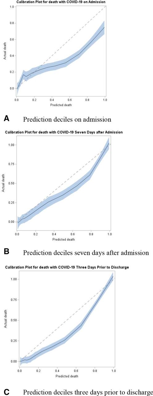
Calibration plots using time-vary model on test set (A) on admission, (B) 7 days after admission and (C) 3 days before discharge (N=864). The plots show a slight propensity for the model to over predict during various points of patients’ stays.

Proportion of actual mortality by predicted mortality score decile ranking in imputed test set. (A) On admission, (B) 7 days after admission and (C) 3 days before discharge (N=864). The model shows an increase in actual mortality among decile groups with higher predicted mortality.
Variable importance
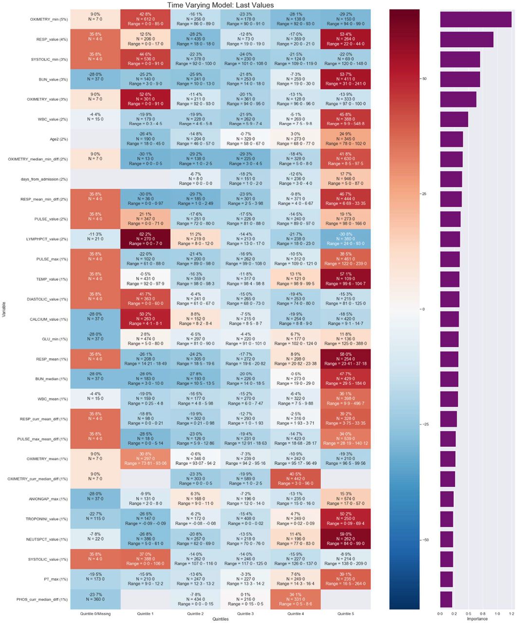
The prediction scores of the model ranged from 0% to 100% with 142 features important to the model. We explored the important feature results using variable importance.15 Figure 4 shows a heat map of the 30 features most associated with the mortality and the overall per cent association on patient’s information on discharge day from the validation and test set combined. It lists the important features along with a calculation of the average change in prediction score of patients for each of level of the feature. Briefly, variable importance varies between zero and one, with higher values indicating features associated more strongly with predictions. Some important features identified by the model included the difference between two values which is results in weight the changes in a patient’s value rather than population. The features of pulse oximetry, respirations, systolic blood pressure, blood urea nitrogen, white blood cell, age, length of stay and lymphocyte per cent had a relative importance of at least 2%. On average, patients had at least a 50% increase in their prediction score if they had any of the following characteristics compared with not having it: respirations ranging 22–44, blood urea nitrogen >31, oximetry value <91%, lymphocyte per cent ranging <7, temperature >99.6, calcium ranging 4.1–8.1, mean respirations ranging 23.4–37.2, troponin value 0.09–69.4 and neutrophil percentage ranging 84–99. Conversely, patients with a median-min difference in oximetry value of 0–0.5, respiratory mean-min difference of 0–0.97 or lymphocyte per cent of 24–93 had at least a 20% decrease in their prediction for mortality.

Ranking of most important 30 of 142 features of the final selected model based on per cent relative importance of the last lab value available in the test set. The purple graph on rightmost column of figure displays the variable importance value. The map also lists the average influence of a feature’s level on a patient’s overall prediction score with darker red boxes and darker blue boxes indicating an increase and decrease in the prediction, respectively (N = 864). Full map in supplemental material.
Discussion
This study describes the development of a machine learning model to predict mortality of patients who present and are admitted to the hospital with a confirmed COVID-19 by PCR and provide an accurate daily risk estimate during the patient’s stay. The aim of this study was to explore and compare three methods to build a model that could accurately predict risk of death on admission and at each day during the stay of the patient.
A strength of the current study was the use over 3000 discharges in a US population. We plan to apply this model to data exported out of clarity each day and provide clinician with daily prediction estimates. The model can be found at Zenodo, along with a sample table that is created prior to applying the model. Unlike other models, it does not require manual calculation of a score, a welcome improvement for the busy clinician. Because the model has high accuracy and is well calibrated, it can be used in other studies as an objective estimation of disease severity. The objective nature of the model is important as it limits biases from documentation issues of overwhelmed clinicians and differences in treatments and provides transparent objective data to characterise severity of a novel disease. Additionally, novel feature engineering methodologies were included such as changes in laboratory/vital results within the context of an individual patient, rather than in the population only, which helped to improve the model’s predictions over the course of a patient’s stay.
Prior studies suggest AI has been slowly gaining traction in healthcare due to the perception that machine learning models are ‘black boxes’ or not interpretable by the user.16 The methods demonstrated in this study are more approachable and easily understood by the clinician. This study presented calibration via deciles that is more intuitive for the non-data scientist. Also, a heat map was created to present results from the variable importance algorithm—the distribution of prediction estimates across the binned variables. Users might hesitate to rely on AI for decisions without knowing the risk factors driving the model, despite the computer making accurate recommendations. By providing user’s information about the model such as variable importance, the association of each feature level with the outcome provides additional insights serve to facilitate trust that is needed to increase the adoption of AI in the healthcare industry.
This model highlights individualised current and prior laboratory and vital results to determine patient-specific mortality risk. Important determinants of risk are further evaluated to illustrate the changes in prediction among patient populations. The interpretability of the model in this study serves to provide insights to intensivists, researchers and administrators of predictors for survivability from a disease with unpredictable or little known outcomes.
This retrospective study applied machine learning algorithms to structured patient data from the EHR of a large urban academic health system to create a risk prediction model to predict mortality during admission in patients with confirmed COVID-19. With an AUC of 0.83 at admission, and 0.97 3 days prior to discharge on imputed data, the model discriminates well and is well calibrated. Additionally, the final model’s AUC was consistent on both the time held out internal validation and external test sets, which gives more confidence the model will continue to perform well on future data. Because we continue to have large amounts of discharges daily, potential changes in populations and modification of treatment protocols, we plan to continue to monitor performance and retrain model when discrimination falls below 0.8. Ideally, the monitoring of the AUC score should be automated and alert the data scientist when the value falls below a predefined threshold. Hospitals should consider developing their own mortality prediction models based on their specific cohorts, as patient populations may differ across facilities therefore affecting validation results.17
Finally, and perhaps most importantly, implementation plays a critical role in supporting in the adoption of AI as healthcare systems face increasingly dynamic and resource-constrained conditions.18 ,19 While a plethora of literature exists addressing data acquisition, development and validation of models, the application of AI in a real-world healthcare setting has not been substantially addressed.20 ,21 22 Often, prediction model results are used to risk adjust and benchmark rates of an outcome.23–25 In addition to using prediction estimates as part of a tool, we suggest models be used as tool in the process of understanding and studying a disease.
Limitations/next steps
The usual limitations associated with an EHR might affect our model. While this model relies on mostly objective data, some inherent bias might be introduced in terms of demographic and laboratory/vital collection and documentation. For example, certain laboratory tests might be ordered on sicker patients or certain types of clinicians might use similar ordering practices that would bias the model. Therefore, the model might be relying on the subjective nature of a clinician rather than purely objective data. On a similar note, patients that might have died after discharge would bias the model. As suggested earlier, results from the model may not be generalisable to other institutions or patient populations; therefore, hospitals should develop tailored models for their own patient population, especially for a disease that is not yet well understood. Because of this, the ‘external validation’ dataset in this study does not meet the TRIPOD definition as it is using a sample from the same patient population although future population. Furthermore, models need to be continually monitored and retrained when performance degrades. Lastly, this model intends to allocate resources, ensure basic and routine care is completed and quantify the health of a patient.
The prediction estimates can be used to create reports adjusting mortality rates by physician, ward or hospital facility. The estimates can also be used to identify high performers to gain insights on potential successful aspects of their care and treatment. The model can be further enhanced by predicting patients who are most likely to unexpectedly expire to gain more insights on how predictors compare with current model. The estimates can also be used for other studies where an objective metric for disease severity is needed. Finally, prediction estimates can be incorporated into an AI tool that can allow clinicians facing a new illness with an uncertain course to identify and prioritise patients who might benefit from targeted, experimental therapy.
Conclusion
Hospitals can develop customised prediction models as the amount of EHR data increases, computing power and speeds are faster and machine learning algorithms are broadly accessible. During times of high demand and large uncertainty around a disease, prediction models can help to identify underlying patterns of predictors of disease and be deployed. This study shows how to build a prediction model whereby the predictions improve during the patient’s course of stay. Results from a highly accurate model can serve as an objective measure of disease severity where manual review of every cases is not feasible. Similar to other industries, machine learning should be integrated into research and healthcare workflows to better understand and study a disease as well as be incorporated into tools to assist in care, allocate resources and aid in discharge decisions to hopefully save lives.
Data availability statement
No data are available. The raw data are not available; however, the model is available at Zenodo (in citation of manuscript).
Acknowledgments
The authors would like thank to Dr Levi Waldron for his general guidance and mentorship on methodology.
References
Supplementary materials
Supplementary Data
This web only file has been produced by the BMJ Publishing Group from an electronic file supplied by the author(s) and has not been edited for content.
Footnotes
Contributors All of the authors were involved in the conception and design of the study, the acquisition of data, the analysis or interpretation of data, and drafting and critical revision of the manuscript for important intellectual content. All approved the final version submitted for publication. AS had full access to the data in the study and takes responsibility for the integrity of the data and accuracy of the data analysis. This study was approved by the NYU Grossman School of Medicine Institutional Review Board (No i20-00671_MOD02), which granted both a waiver of informed consent and a waiver of the Health Information Portability and Privacy Act.
Funding The authors have not declared a specific grant for this research from any funding agency in the public, commercial or not-for-profit sectors.
Competing interests None declared.
Provenance and peer review Not commissioned; externally peer reviewed.
Supplemental material This content has been supplied by the author(s). It has not been vetted by BMJ Publishing Group Limited (BMJ) and may not have been peer-reviewed. Any opinions or recommendations discussed are solely those of the author(s) and are not endorsed by BMJ. BMJ disclaims all liability and responsibility arising from any reliance placed on the content. Where the content includes any translated material, BMJ does not warrant the accuracy and reliability of the translations (including but not limited to local regulations, clinical guidelines, terminology, drug names and drug dosages), and is not responsible for any error and/or omissions arising from translation and adaptation or otherwise.