Opening the black box of neural networks: methods for interpreting neural network models in clinical applications
Introduction
Artificial intelligence (AI) methods, especially those based on machine learning methods, are rapidly becoming essential for analysis of complex clinical and other data, and for decision support in the clinic (1-4). Artificial neural networks (ANNs) are highly parameterized, non-linear models with sets of processing units called neurons that can be used to approximate the relationship between input and output signals of a complex system (5). While ANNs can be used as powerful predicting tools compared to more conventional models (e.g., linear regression), they are also criticized as ‘black boxes’. Compared to linear methods, ANN models are very difficult to interpret and it is challenging to identify which descriptors (predictors) are the most important and how they are related to the property being modeled. The hyper-parameterized structure of neural networks creates complex functions from the input that can approximate observed outcomes with minimal error (6). As such ANNs can approximate any continuous function, as postulated by the Universal Approximation Theorem, but the immediate structures of a fitted model do not provide insights into the relative importance, underlying relationships, structures of the predictors or covariates with the modelled outcomes.
As an example, neural networks can be used to predict clinical deterioration in adult hematologic malignancy patients (7). The input is a set of predictors P (diastolic blood pressures, heart rate, white blood cell count, etc.) and the output is an outcome O (ICU transfer, cardiac arrest, discharge). The neural network model finds a mathematical function f (P) =O, where f can be arbitrarily complex, and might change according to the sample of the study population. The black box issue is that the approximation given by the neural network will not provide insight into the form of f as there is often no simple relationship between the network weights and the property being modeled. Even the analysis of the relevance of input variables is challenging (8), and neural networks do not generate a statistically identifiable (deterministic) model. For a given training dataset and network topology, there can be multiple neural networks with different weights that generate very similar predictions of the modeled property, complicating understanding of the ANN and relevant predictors. In contrast, a generalized regression model is an example of the “non-black box models”, generating interpretable models with reproducible regression coefficients and a closed form function f where the importance of each predictor is explicitly and clinically interpretable.
Recognizing the issue, many methods have been developed to help subject-matter audiences to understand the underlying functions of ANN. This article provides an overview of several of the most common algorithms and illustrates how they perform using examples. The R statistical programming language (version 3.4.3) is used in the following examples.
Working example
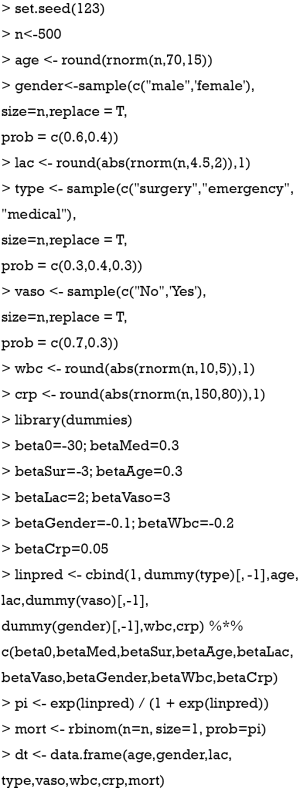
An artificial data set that mimics a clinical situation was generated for the examples.
The above code generates seven predictors (descriptors): age, gender, lactate (lac) type of patients type (type), use of vasopressor (vaso), white blood cell count (wbc), and C-reactive protein (crp). The mortality (mort) is binary clinical outcome variable which takes two values 0 for alive and 1 for deceased. The relationship between mort and predictors are built under the logistic regression model framework. However, we will build a neural network model in the following example.
Fitting a neural network model
There are several types of machine learning methods that could be used to generate models but we use a neural network model in our examples. Several packages are available in R to develop an ANN. The nnet package (version 7.3-12) is widely used and can fit a single-hidden-layer neural network (9). The caret (Classification And Regression Training) package (version 6.0-78) contains a set of tools for building machine learning models in R (10).
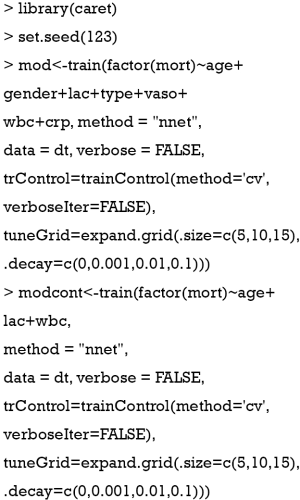
The above code fits two neural network models. The first one model mod is fit with the train() function using all seven predictors. In the model, cross validation is used to select the best model by tuning the parameters size and decay. In general, the size parameter defines the number of hidden nodes in the network, which are essentially free parameters that allow flexibility in the model fit between input and output layers. Increasing the number of hidden nodes increases the flexibility of the model but at the risk of over-fitting. The decay parameter is more abstract, in that it controls the rate of decay for changing the weights as used by the back-propagation fitting algorithm. This also affects how regular or irregular the weights can be relative to each other—with potential for over-fitting and/or increasing non-linearity in the fit. In the example, the number of hidden units (size parameter) is chosen from 5, 10 and 15, and the decay parameter is chosen from 0, 0.001, 0.01, and 0.1, depending on which model has the best accuracy. More details of how the train() function works with neural network model can be found at http://topepo.github.io/caret/ . The second model, modcont, contains only continuous variables as the predictors including age, lac and wbc.
Variable importance using Garson’s algorithm
The weights connecting neurons in an ANN are partially analogous to the coefficients in a generalized linear model. The combined effects of the weights on the model predictions represent the relative importance of predictors in their associations with the outcome variable. However, there are many weights connecting one predictor to the outcome in an ANN. The large number of adjustable weights in an ANN makes it very flexible in modeling nonlinear effects but imposes challenges for the interpretation. Garson proposed that the relative importance of a predictor can be determined by dissecting the model weights (11,12). All connections between each predictor of interest and the outcome are identified. Pooling and scaling all weights specific to a predictor generates a single value ranging from 0 to 1 that reflects relative predictor importance. The relative importance can be computed in R with the NeuralNetTools (version 1.5.1) package (13).
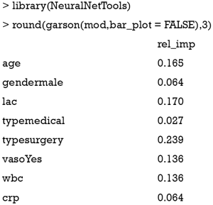
The relative importance of each predictor is shown in the above output. The results suggest that surgery type is the most important predictor of mortality outcome, followed by lactate (lac) and age. The relative importance of each predictor can be plotted by setting the bar_plot argument to TRUE (the default setting in the garson() function).
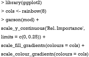
Figure 1 displays the relative importance of each predictor. The garson() function returns a ggplot object (14), and the default aesthetics can be further modified with the following code.
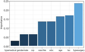
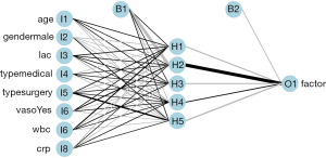
Figure 2 shows how the plot aesthetics can be changed from the default output of the garson() function. Furthermore, the neural network model can also be visualized with the plotnet() function.
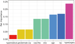
Figure 3 is a diagram of the neural network architecture. The black lines indicate positive weights and grey lines indicate negative weights. Line thickness is in proportion to the relative magnitude of each weight. The first layer receives the input variables (I1 through I8) and each is connected to all nodes in the hidden layer (H1 through H5). The output layer (O1) is connected to all hidden layer nodes. Bias nodes provide a function that is similar to the intercept term in a linear model and are shown as connections to the hidden and output layers in the plot.
Sensitivity analysis using the Lek’s profile method
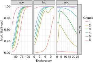
The Lek’s profile method can be used to explore the relationship between the outcome variable and a predictor of interest, while holding other predictors in a set of constant values (e.g., minimum, 20th quantile, maximum) (15,16). The relationship between an outcome and a predictor might differ given the context of the other predictors (i.e., the presence of an interaction) and the sensitivities may vary at different points of the surface given the ability of the model to describe nonlinear relationships. In essence, the method generates a partial derivative of the response with respect to each descriptor and can provide insight into these complex relationships described by the model. The Lek’s profile method is only applicable to models with continuous explanatory variables, so the modcont model is used for illustration.
Figure 4 shows output from Lek’s profile method using the lekfrofile() function in the NeuralNetTools package. By holding other predictors at their minima, at 20th, 40th, 60th, 80th quantiles, and at their maximum (6 groups in the figure), the relationships between the outcome probability and predictor of interest varies widely for the variable wbc.
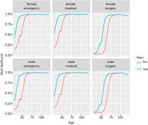
If there are categorical (discrete) variables in a given dataset, the following code can be used to look at the model response across the range of values for one explanatory variable at a time. The final plot was created using facets for selected levels of the discrete explanatory variables. You can specify which continuous explanatory variable to evaluate with the varex object and you can change the quantile at which the other explanatory variables are held constant using the quant object.
The %>% operator is read as “and then”, and is piping an object forward into a function or call expression (17). Figure 5 shows Lek’s profile method for the predictor age at all combinations of other discrete variables. There are 2×2×3=12 curves, e.g., there are 2 levels for gender, 3 levels for type and 2 levels for vaso. Continuous variables are held at their median, generating only 1 level.
Partial dependence plot
Partial dependence of an outcome variable on a predictor of interest can be calculated as follows (18):
- Suppose there are k observations, and i
 {1,2,3,...,k}. The variable of interest is denoted as x1, with distinct values of {x11,x12,...,x1k}. The original values of x1 in the training dataset are replaced with the constant x1i.
 - Compute the predicted values of an outcome variable from the modified training dataset.
- The average prediction for x1 is computed as
 .
. - The partial dependence plot is to plot the pairs
 for i ={1,2,3,...,k}.
The plot for a single predictor can be created with the pdp package (version 0.6.0) (18).
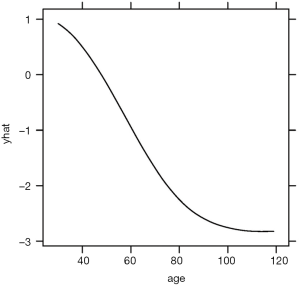
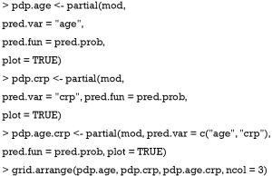
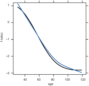
The above code loads and attaches the pdp and viridisLite packages to the R workspace. The viridisLite package (version 0.3.0) helps to design color maps which are perfectly uniform, both in regular form and also when converted to black-and-white. The package is also designed to aid perception by readers with the most common form of color blindness. The output in Figure 6 shows the relationship between age and yhat. The response variable is shown in logit scale.
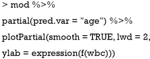
The plotPartial() function is used to display a more detailed partial plot. It operates on objects returned by the partial() function and provides many options to modify the plot. The above example shows how to add a LOESS smooth line to the plot (Figure 7).
The pdp package can also be used to plot the response variable and two predictors as a 2-D or 3-D plot. Fortunately, the pdp package makes this work easy.
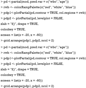
To investigate the simultaneous effect of two predictors on the predicted outcome, the pred.var argument in the partial() function takes a 2-element string vector indicating the names of the predictors of interest. In the second line, the colorRampPalette() function interpolates a set of given colors to create new color palettes. The first plot, pdp1, is a 2-D contour plot that was created by setting the contour argument to TRUE. The second plot, pdp2, is a 3-D surface plot that is created by setting the levelplot argument to FALSE. Finally, the grid.arrange() function combines the two plots into a single image (Figure 8) arranged in a 1×2 matrix (19).
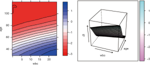
However, the above figures display the outcome variable on a linear scale, which is not interpretable for most subject-matter audiences. The probability of the outcome can be displayed by specifying a function for the transformation from logit space to a probability.
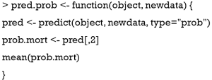
There are two arguments for the pred.prob() function. The first argument is the object that receives the trained ANN. The second argument is newdata as an optional set of data to predict. If newdata is not specified, the original dataset is used for prediction. The type argument in the predict() function can be either “raw” or “prob”. In this case, “prob” is used to return class probability. The following code plots the partial dependence plots and combines them into one using grid.arrange().
It is noted that the y-axis is now on a probability scale (Figure 9).
Local interpretable model-agnostic explanations (LIME)
LIME can be used to explain the predictions of any classifications or regressions, by approximating it locally with an interpretable model (20). The “agnostic” descriptor suggests that the tool can be used to provide insight into a process that “is not known or cannot be known”, which is especially relevant to the “black box” characteristics of a neural network model. Essentially, LIME can be used to interpret complex models by providing a qualitative link between the input variables and the response. This is accomplished by dissecting and locally approximating the larger model with simpler models, such as linear or decision tree models, that are conceptually easier to understand and interpret. The lime package (0.4.0) is used to perform the LIME algorithm (21).
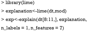
The lime() function is the core function of the package. The first argument is the training data, which is the dt dataset used to create the models in the above examples. The second argument is the neural network model mod that need to be explained. The lime() function returns an explainer object that is passed to the explain() function. The explain() function takes new observations (e.g., patients 8 to 11 in the example data) along with the explainer object and returns a matrix with prediction explanations, one observation per row. The returned explanations can then be visualized with several plot functions provided by the lime package.
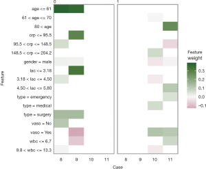
The plot_explanations() function draws a facetted heatmap-style visualization of all case-feature combinations (Figure 10). The case numbers are shown in the horizontal axis and categorized features are displayed in the vertical axis. There are two types of outcome events for mortality, denoted as 0 and 1 in the right and left panels, respectively. Cases 8 and 9 are survivors (mort =0) and cases 10 and 11 are non-survivors (mort =1). Feature weights are shown with the colors. Positive (green) weights suggest a feature is supporting the outcome, and negative (red) weights suggest a feature is contradicting the outcome. In the example, age younger than 61 is shown in green for survivors (left panel) and negatively associated with mortality. In contrast, use of vasopressor (vaso = yes) is red in the left panel and green in the right panel, and is a risk factor for death. This plot is important for the understanding of how the ANN makes predictions. Clearly, Clinicians reserve their own judgements in decision making, but the interpreted neural network models that predict patient outcomes (e.g., patient very likely to die because he/she is very old and uses vasopressors) can be critically important supporting element of the overall decision process.
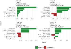
Finally, the supporting and contradicting features to make a mortality prediction can be plotted for each patient with the plot_features() function. The function requires only the explanation output and number of columns as input arguments. The feature plot is shown in Figure 11.
Discussion
Due to their “black-box” nature, many machine learning methods suffer from the limitation of providing meaningful interpretations that can enhance understanding in subject-matter research. This article reviewed and demonstrated several methods to help clinicians understand neural network models of important patient parameters and outcomes. One or several of the illustrated methods will be suitable for essentially any type of clinical outcome model. Applicability of interpretation algorithms may be somewhat case dependent. The methods suggested in this review can be applied to ANN, random forest and many other black-box types of methods. The step-by-step instructions and R code provided herein offer an approach for researchers to open the black-box by providing visual presentations and clear interpretations of the analysis results.
This work has a few limitations. First, the recommended methods only present the predicted means, but not the corresponding level of uncertainty. Second, we focus on reviewing useful tools to facilitate interpretation of the results. The technical details related to the model evaluation, and cross-validation, and techniques to avoid overfitting were not discussed. At last, prediction models are fundamentally different from explanatory models. The interpretation of the results obtained from a prediction model reflects the association between the predictor and the outcome after adjustment of other covariates included in the same model. It may not directly offer causal interpretation.
Acknowledgements
Funding: Z Zhang received funding from the Public Welfare Research Project of Zhejiang Province (LGF18H150005) and Scientific Research Project of Zhejiang Education Commission (Y201737841).
Footnote
Conflicts of Interest: The authors have no conflicts of interest to declare.
References
- Smalley E. AI-powered drug discovery captures pharma interest. Nat Biotechnol 2017;35:604-5. [Crossref] [PubMed]
- Hamet P, Tremblay J. Artificial intelligence in medicine. Metab Clin Exp 2017;69S:S36-S40. [Crossref] [PubMed]
- Ryu JY, Kim HU, Lee SY. Deep learning improves prediction of drug-drug and drug-food interactions. Proc Natl Acad Sci USA 2018;115:E4304-11. [PubMed]
- Zhu B, Liu JZ, Cauley SF, et al. Image reconstruction by domain-transform manifold learning. Nature 2018;555:487-92. [Crossref] [PubMed]
- Stefaniak B, Cholewiński W, Tarkowska A. Algorithms of Artificial Neural Networks - Practical application in medical science. Polski Merkuriusz Lekarski 2005;19:819-22. [PubMed]
- Hornik K. Approximation capabilities of multilayer feedforward networks. Neural Networks 1991;4:251-7. [Crossref]
- Hu SB, Wong DJL, Correa A, et al. Prediction of Clinical Deterioration in Hospitalized Adult Patients with Hematologic Malignancies Using a Neural Network Model. PLoS One 2016;11:e0161401. [Crossref] [PubMed]
- May R, Dandy G, Maier H. Review of Input Variable Selection Methods for Artificial Neural Networks. In: Artificial Neural Networks - Methodological Advances and Biomedical Applications. InTech, 2011.
- Venables WN, Ripley BD. Modern Applied Statistics with S [Internet]. Forth. Springer, 2002. Available online: http://www.stats.ox.ac.uk/pub/MASS4
- Kuhn M. caret: Classification and Regression Training. Available online: https://CRAN.R-project.org/package=caret. 2017.
- Garson GD. Interpreting neural network connection weights. Artificial Intelligence Expert 1991;6:46-51.
- Goh ATC. Back-propagation neural networks for modeling complex systems. Artificial Intelligence in Engineering 1995;9:143-51. [Crossref]
- Beck M. NeuralNetTools: Visualization and Analysis Tools for Neural Networks. Available online: https://CRAN.R-project.org/package=magrittr. 2018.
- Wickham H. ggplot2: Elegant Graphics for Data Analysis. Springer International Publishing, 2016.
- Lek S, Delacoste M, Baran P, et al. Application of neural networks to modelling nonlinear relationships in ecology. Ecological Modelling 1996;90:39-52. [Crossref]
- Gevrey M, Dimopoulos I, Lek S. Review and comparison of methods to study the contribution of variables in artificial neural network models. Ecological Modelling 2003;160:249-64. [Crossref]
- Bache SM, Wickham H. magrittr: A Forward-Pipe Operator for R. Available online: https://CRAN.R-project.org/package=magrittr. 2014.
- Greenwell BM. pdp: An R Package for Constructing Partial Dependence Plots. The R Journal 2017;9:421-36.
- Auguie B. gridExtra: Miscellaneous Functions for “Grid” Graphics. Available online: https://CRAN.R-project.org/package=gridExtra. 2017.
- Ribeiro M, Singh S, Guestrin C. “Why Should I Trust You?”: Explaining the Predictions of Any Classifier. Stroudsburg, PA, USA: Association for Computational Linguistics, 2016:97-101.
- Pedersen TL, Benesty M. lime: Local Interpretable Model-Agnostic Explanations. Available online: https://CRAN.R-project.org/package=lime. 2018.




 {1,2,3,...,k}. The variable of interest is denoted as x1, with distinct values of {x11,x12,...,x1k}. The original values of x1 in the training dataset are replaced with the constant x1i.
 .
. for i ={1,2,3,...,k}.
